2312
I just finished the sci-fi novel 2312 by Stanley Kim Robinson. Like most novels over 500 pages, I thought it could be shorter. However, I enjoyed Robinson’s ambitious vision of the future and the care he takes in world-building. What makes the story ambitious is that he developed not a single world but several worlds.
The story centers around the events of year 2312. In the past 200 or so years humans colonized the solar system. There are human settlements on all the terrestrial planets as well as mid-size moons on Jupiter and Saturn such as Io and Titan. Humans were forced from their native Earth due to calamitous environment conditions. This plot device is a well-worn sci-fi trope. However, what Robinson adds to the genre is a carefully crafted inter-planetary society with intricate social, economic and political relations.
Earth of course is seen by those who colonized space (“spacers”) as the center of pestilence in the solar system characterized by widespread poverty and inequality. There is still a market economy on Earth, whereas the nations that are part of an interplanetary organization called the Mondragon benefit from a planned economy that guarantees the essentials necessary to exist in space. Earth, however, is still the center of political and financial power in the solar system, so each space settlement must maintain political relations with the planet. The exception is Mars, which earned a degree of freedom after staging the first inter-planet revolution for independence.
Essential to the colonization of the solar system are qubes. These are quantum computers that are able to perform enormous computational tasks such as planning the space economy. Ownership of these computers are a source of power in the solar system and perpetuate a kind of computational arms race between the major solar system powers.
There are a host of other technological advances that allow for humans to thrive in space such as terraforming and biotechnology that enables long human lifespans. However, I found the economic and political relationships between the colonies the most interesting part of the novel. Some settlements relied on exporting nitrogen to other planets, while others like Mercury relied on supplying sunlight to outposts near the outer reaches of the solar system.
The book alludes to many astrological bodies in our solar system and I repeatedly consulted Wikipedia to check the location of these bodies and how big they are. This Wikipedia page in particular was a great source of information. I had the idea to scrape information from this page using Python and analyze the data using R. Below, I create graphs to compare the physical properties of the main bodies in the solar system. I then see how well kmeans clustering performs in grouping these celestial objects together.
Our Solar System
I scrape the first table on the webpage under the heading List of objects by radius and the subheading Larger than 400 km. This table includes multiple measures of the radius, volume, mass and gravity of different astronomical objects, as well as their shape, type and density. Below is the Python code to scrape the information and build the dataset:
from requests import get
from bs4 import BeautifulSoup
import json
import numpy as np
import xlsxwriter
#scrape table
url = 'https://en.wikipedia.org/wiki/List_of_Solar_System_objects_by_size'
response = get(url)
html_soup = BeautifulSoup(response.text, 'html.parser')
entire_table = html_soup.find("table",{"class":"wikitable sortable"})
all_rows = entire_table.find("tbody").find_all("tr")
#loop to create dataframe
table_columns = ['body','image','radius_km','radius_r','volume_km',
'volume_v','mass_kg','mass_m','density','gravity_ms',
'gravity_g','type','shape','number']
jsonList = []
for row in all_rows[2:len(all_rows)-2]:
    rowList = []
    for cell in row.find_all('td'):
        rowList.append(cell.text)
    currJson = dict(zip(table_columns,rowList))
    jsonList.append(currJson)
full_df = pd.DataFrame(jsonList)
#process dataframe
df = full_df
##strip whitespace and paragraph characters, remove commas
df = df.apply(lambda x: x.str.strip() if x.dtype == "object" else x)
df = df.apply(lambda x: x.str.strip('\n\t') if x.dtype == "object" else x)
df[list(df.columns)] = df[list(df.columns)].replace({',': ''}, regex=True)
##process radius_km with regex
df.radius_km = df.radius_km.apply(lambda x: x.split("♠")[1])
def regex_func(x):
    x = re.sub("[\(\[].*?[\)\]]", "", x)
    return(x)
df.radius_km = df.radius_km.map(regex_func)
df = df.apply(lambda x: x.map(regex_func) if x.dtype == "object" else x)
I then clean up the data and build plots using R. Since including all of the code in the post makes it very long, I’ll include only the code to build the scraper and leave out the R code. However, you can find all of the code here.
We begin with a look at average metrics for each type of astronomical object:
We can make a few easy inferences. By far the most massive object type is “star”. The sun is a mind-boggling 333,000 times as massive as the Earth, has a radius that is about 109 times as wide as the Earth’s and has a force of gravity that is nearly 28 times the Earth’s gravity. The gas and ice giants are also astoundingly large in terms of mass and size compared to Earth. However, the four terrestrial planets constitute the densest objects in the solar system. Together, their average density is five times that of the gas giants.
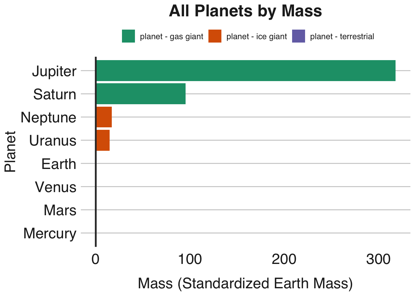
The following plot illustrates how massive the planets in our solar system are:

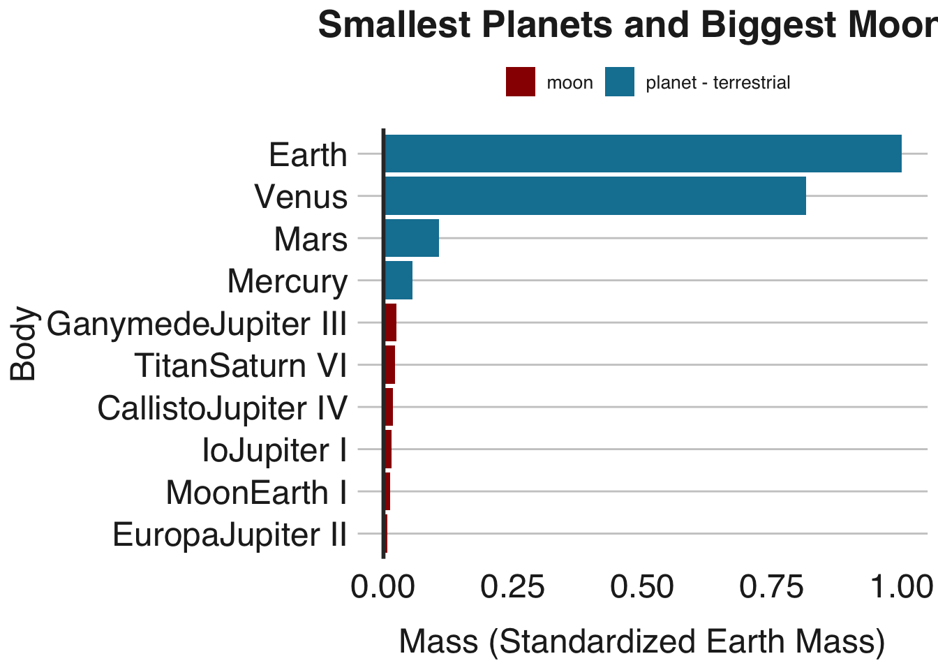
Together the gas giants Jupiter and Saturn are about 206 times as massive as the Earth, while the ice giants Neptune and Uranus are about 15 times as massive. However, this plot shows just how much more massive Jupiter is than the rest of the planets in our solar system. We can barely make out the masses of the four terrestrial planets when compared to the four giants. Below, we compare masses of the four terrestrial planets to the six most massive moons in the solar system:

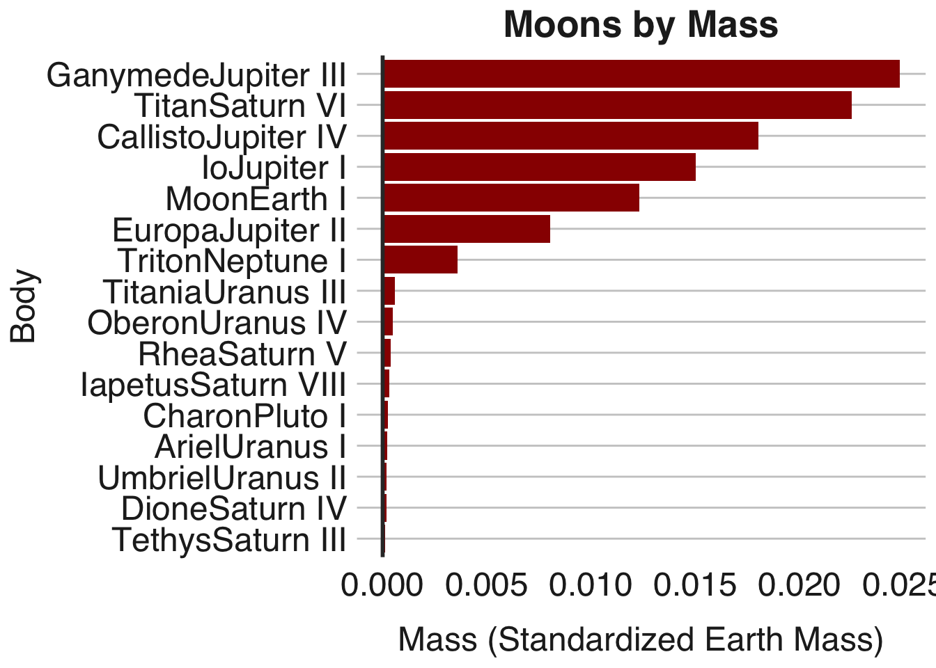
Of course, these bodies are where most of the action in 2312 takes place. Venus and Mars were terraformed successfully, while the main character Swan lives on Mercury in a city called Terminator which constantly moves on tracks to stay out of the sun. Mercury’s proximity to the sun prevents it from being terraformed. However, the other main character Wahram lives on a Saturnian moon settlement on Titan and there are is also a human settlement on the Jovian moon Io. Below is a list of all the moons in our solar system by mass:

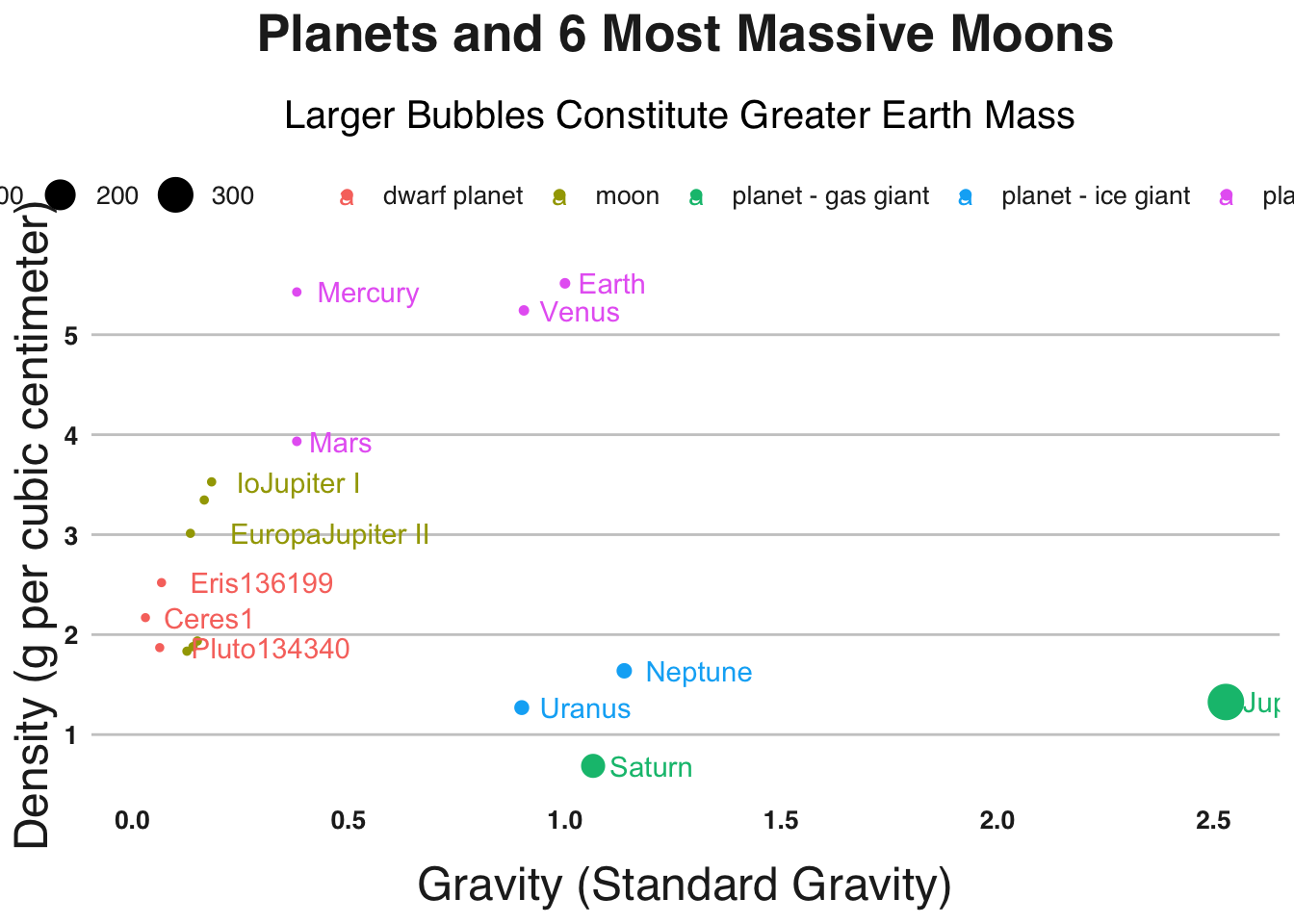
So far we’ve only looked at mass. Below we plot each object’s gravity on the x-axis and each object’s density on the y-axis. The size of each dot is proportional to each object’s mass and the color of each dot is the object type.

There appear to be natural groups that emerge when we plot the objects this way. The terrestrial planets cluster in the upper left quadrant, the dwarf planets cluster in the lower left quadrant and the giant planets settle towards the lower center of the graph.
While we can tease out these relationships graphically, this dataset lends itself well to cluster analysis. Using the five metrics I display in the first table above, I use kmeans to cluster all of the 28 bodies for which we have full data. Kmeans is a quantitative approach to teasing out the relationships between the bodies that we see visually in the graph. If we are able to identify the type of astronomical body simply by these metrics, we will see perfect separation into the 5 object types. However, the kmeans clustering yields imperfect—albeit interesting—results. I manually name the new clusters that kmeans yields based on the majority of the objects in each cluster. Here is the breakdown by the cluster type:
##
##                        big moons/dwarf planets gas giants mid-sized moons
##   dwarf planet                               3          0               0
##   moon                                       8          0               3
##   planet - gas giant                         0          2               0
##   planet - ice giant                         1          0               0
##   planet - terrestrial                       0          0               1
##   star                                       0          0               0
##
##                        small moons star terrestrial planets
##   dwarf planet                   0    0                   0
##   moon                           5    0                   0
##   planet - gas giant             0    0                   0
##   planet - ice giant             1    0                   0
##   planet - terrestrial           0    0                   3
##   star                           0    1                   0
Here is the full list of each body by their type and the cluster’s type:
There are two groups that kmeans identifies without a problem. The sun is so different from the other objects that kmeans isolates it easily. The same goes for the two gas giants. Out of the terrestrial planets, we are able to group Mercury, Venus and Earth together successfully. However, as the graph hinted above, kmeans groups Mars with the mid-sized moons Io, Europa and our very own Luna. This is not so strange given that Mars is actually much less dense than the other terrestrial planets. In fact, it’s density is closer to Io’s than it is to any of three other terrestrial planets.
The biggest blunder that kmeans commits is its inability to properly classify the ice giants. Though on the graph they appear to be closer to the gas giants in terms of mass and density, kmeans groups Uranus with the small moons and Neptune with the big moons and dwarf planets. While the algorithm correctly identifies their mass and volume as distinguishing features for the ice giants, the two planets’ density and gravity are different enough that kmeans cannot make the leap of grouping them together. However, the algorithm does a good job in grouping all of the dwarf planets together. Its decision to group together dwarf planets and big moons is not so off-base either given that the big moons and dwarf planets share very similar masses and volumes.
Despite its misclassification of the ice giants, the algorithm reveals interesting commonalities between the bodies in our solar system. For instance, in 2312 Mars is a completely terraformed planet but Mercury is not. Kmeans grouped Mars with mid-sized moons like Io, Europa and our moon. This is a fitting choice. In the story Robinson alludes to discussions in the solar system over whether or not terraforming should commence on these three moons. Perhaps the algorithm picked up on these lunar objects’ shared potential for terraforming. This potential eluded us, but was perhaps evident to Robinson when writing his story.